Excess rentals in Transport for London bike sharing
1. Summary and preview of the dataset
url <- "https://data.london.gov.uk/download/number-bicycle-hires/ac29363e-e0cb-47cc-a97a-e216d900a6b0/tfl-daily-cycle-hires.xlsx"

# Download TFL data to temporary file
httr::GET(url, write_disk(bike.temp <- tempfile(fileext = ".xlsx")))
## Response [https://airdrive-secure.s3-eu-west-1.amazonaws.com/london/dataset/number-bicycle-hires/2022-09-06T12%3A41%3A48/tfl-daily-cycle-hires.xlsx?X-Amz-Algorithm=AWS4-HMAC-SHA256&X-Amz-Credential=AKIAJJDIMAIVZJDICKHA%2F20220915%2Feu-west-1%2Fs3%2Faws4_request&X-Amz-Date=20220915T093323Z&X-Amz-Expires=300&X-Amz-Signature=cc365f0b7c63fbb3c569555241c889e93dc934693bd61c55a9c211c71afcc438&X-Amz-SignedHeaders=host]
## Date: 2022-09-15 09:33
## Status: 200
## Content-Type: application/vnd.openxmlformats-officedocument.spreadsheetml.sheet
## Size: 180 kB
## <ON DISK> /var/folders/6g/_mjhz_m510n4cb504ffpwxh00000gn/T//RtmpEx08Mz/filee726baa1e6f.xlsx# Use read_excel to read it as dataframe
bike0 <- read_excel(bike.temp,
sheet = "Data",
range = cell_cols("A:B"))
# change dates to get year, month, and week
bike <- bike0 %>%
clean_names() %>%
rename (bikes_hired = number_of_bicycle_hires) %>%
mutate (year = year(day),
month = lubridate::month(day, label = TRUE),
week = isoweek(day))
skim(bike)| Name | bike |
| Number of rows | 4416 |
| Number of columns | 5 |
| _______________________ | |
| Column type frequency: | |
| factor | 1 |
| numeric | 3 |
| POSIXct | 1 |
| ________________________ | |
| Group variables | None |
Variable type: factor
| skim_variable | n_missing | complete_rate | ordered | n_unique | top_counts |
|---|---|---|---|---|---|
| month | 0 | 1 | TRUE | 12 | Aug: 403, Jul: 374, Jan: 372, Mar: 372 |
Variable type: numeric
| skim_variable | n_missing | complete_rate | mean | sd | p0 | p25 | p50 | p75 | p100 | hist |
|---|---|---|---|---|---|---|---|---|---|---|
| bikes_hired | 0 | 1 | 26844.3 | 9899.73 | 2764 | 19698 | 26607 | 34206 | 73094 | ▃▇▅▁▁ |
| year | 0 | 1 | 2016.1 | 3.51 | 2010 | 2013 | 2016 | 2019 | 2022 | ▆▅▇▅▇ |
| week | 0 | 1 | 26.6 | 15.01 | 1 | 14 | 27 | 40 | 53 | ▇▇▇▇▇ |
Variable type: POSIXct
| skim_variable | n_missing | complete_rate | min | max | median | n_unique |
|---|---|---|---|---|---|---|
| day | 0 | 1 | 2010-07-30 | 2022-08-31 | 2016-08-14 12:00:00 | 4416 |
glimpse(bike)## Rows: 4,416
## Columns: 5
## $ day <dttm> 2010-07-30, 2010-07-31, 2010-08-01, 2010-08-02, 2010-08-0…
## $ bikes_hired <dbl> 6897, 5564, 4303, 6642, 7966, 7893, 8724, 9797, 6631, 7864…
## $ year <dbl> 2010, 2010, 2010, 2010, 2010, 2010, 2010, 2010, 2010, 2010…
## $ month <ord> Jul, Jul, Aug, Aug, Aug, Aug, Aug, Aug, Aug, Aug, Aug, Aug…
## $ week <dbl> 30, 30, 30, 31, 31, 31, 31, 31, 31, 31, 32, 32, 32, 32, 32…2. Comparison of the actual number of bike rentals per month between 2017-2022 to the expected number of bike rentals per month between 2016-2019
# generate expected bike hired value for each month
bike_expected_month<-bike %>%
  filter(year>= 2016 & year <= 2019) %>%
  group_by(month) %>%
  mutate(expected_month_year=mean(bikes_hired, na.rm = TRUE)) %>%
  summarise(expected_mean=mean(expected_month_year))

# generate real bike hired value for each month in each year
bike_real_month<-bike %>%
  filter(year>=2017 & year<=2022) %>%
  group_by(year,month) %>%
  summarise(actual_hired=mean(bikes_hired))

# combine expected and real bike table
combine = left_join(x=bike_expected_month, y=bike_real_month, by = "month", all.x=TRUE) %>%
   mutate(min_1=pmin(actual_hired,expected_mean)) %>%
   group_by(year)

# graphing ribbon and line
h <- ggplot(combine, aes(x=month))
h+  geom_ribbon(aes(ymin=min_1, ymax=actual_hired ,group=year),fill="chartreuse4",alpha=0.25)+
    geom_ribbon(aes(ymin=min_1, ymax=expected_mean,group=year),fill="red", alpha=0.25)+
    geom_line(aes(y=expected_mean,group=year), color="blue",size=0.8)+
    geom_line(aes(y=actual_hired,group=year),color="black",size=0.2)+
    facet_wrap(~year)+
    labs(
    title = "Monthly changes in TfL bike rentals",
    subtitle = "Change from monthly average shown in blue
and caculated between 2016-2019",
    x = NULL,
    y = "Bike rentals",
    caption="Source: TfL, London Data Store")+
    scale_y_continuous(limits = c(10000,45000))+
    theme_minimal()+
    theme(text = element_text(size = 7))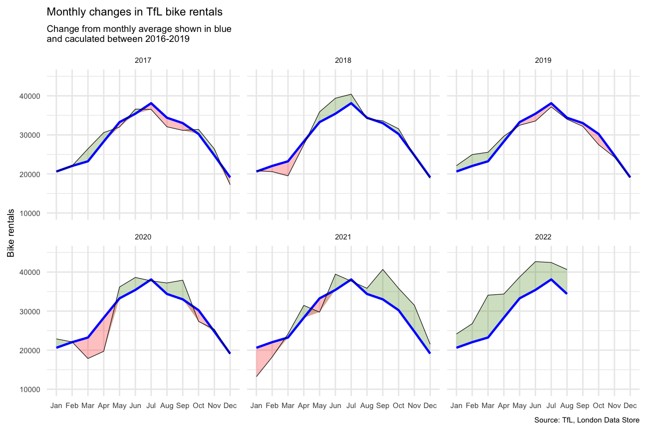
3. Percentage changes between the actual number of bike rentals per week between 2017-2022 and the expected number of bike rentals per week between 2016-2019
# generate expected bike hired value for each week
bike_expected_week<-bike %>%
  filter(year>=2016 & year<=2019) %>%
  group_by(week) %>%
  mutate(expected_week_year=mean(bikes_hired)) %>%
  summarise(expected_mean=mean(expected_week_year))

# generate real bike hired value for each month in each week
bike_real_week<-bike %>%
  filter(year>=2017 & year <=2022) %>%
  group_by(year,week) %>%
  summarise(actual_hired=mean(bikes_hired))

# combine expected and real bike table
combine1 = left_join(x=bike_expected_week, y=bike_real_week, by = "week", all.x=TRUE) %>%
   mutate(change = (actual_hired - expected_mean)/expected_mean, rug_positive=ifelse(change>0, "col1", "col2")) %>%
   group_by(year) %>%
   filter(week < 52)                       # to limited the extreme value(the week 52/53 may cover next year)


# graphing ribbon and rug and line and rect
library(scales)     # library for percentage drawing
options(ggplot2.discrete.colour= c("chartreuse4", "red"))     # set the option for default factor color assignment
h <- ggplot(combine1, aes(x=week), options)
h+geom_ribbon(aes(ymin=pmin(change,0), ymax=0 ,group=year),fill = "red", alpha = 0.25)+
    geom_ribbon(aes(ymin=0, ymax=pmax(change,0),group=year),fill = "chartreuse4", alpha = 0.25)+
    geom_line(aes(y=change,group=year), size = 0.7)+
    geom_rect(aes(xmin=14,xmax=26),fill="grey", ymin=-1,ymax=1.5, alpha=0.01)+
    geom_rect(aes(xmin=40,xmax=52),fill="grey", ymin=-1,ymax=1.5, alpha=0.01)+
    geom_rug(aes(color = rug_positive), show.legend = FALSE)+
    scale_y_continuous(limits = c(-0.55, 1.05),labels = percent)+
    facet_wrap(~year)+
    labs(
    title = "Weekly changes in TfL bike rentals",
    subtitle = "% change from weekly averages
calculated between 2016-2019",
    x = "week",
    y = NULL,
    caption="Source: TfL, London Data Store"
  ) +
    theme_minimal()+
    theme(text = element_text(size = 7))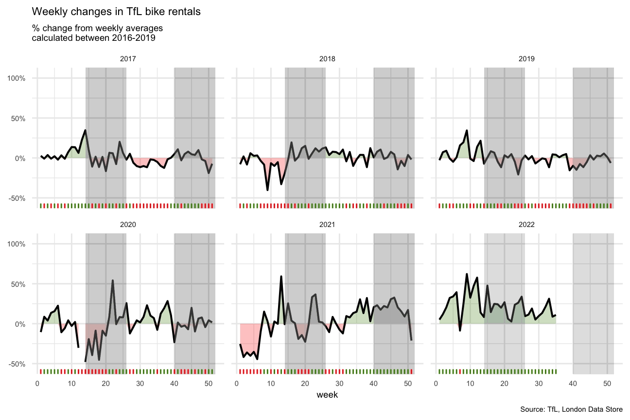
4. Why use mean instead of median to calculate expected rental?
Normally, a mean is used as expected values and in this case, expected rentals. This applies to the cases where the distribution is not extremely unsymmetrical. From the diagrams above, we can see that the distributions are generally symmetrical. If there are cases where the distributions are extremely skewed and have clear outliers, median would be preferred as the value is less distorted.