Differences of IMDB ratings between directors - Steven Spielberg and Tim Burton

1. Summary and preview of the dataset
movies <- read_csv(here::here("data", "movies.csv"))
skim(movies)| Name | movies |
| Number of rows | 2961 |
| Number of columns | 11 |
| _______________________ | |
| Column type frequency: | |
| character | 3 |
| numeric | 8 |
| ________________________ | |
| Group variables | None |
Variable type: character
| skim_variable | n_missing | complete_rate | min | max | empty | n_unique | whitespace |
|---|---|---|---|---|---|---|---|
| title | 0 | 1 | 1 | 83 | 0 | 2907 | 0 |
| genre | 0 | 1 | 5 | 11 | 0 | 17 | 0 |
| director | 0 | 1 | 3 | 32 | 0 | 1366 | 0 |
Variable type: numeric
| skim_variable | n_missing | complete_rate | mean | sd | p0 | p25 | p50 | p75 | p100 | hist |
|---|---|---|---|---|---|---|---|---|---|---|
| year | 0 | 1 | 2.00e+03 | 9.95e+00 | 1920.0 | 2.00e+03 | 2.00e+03 | 2.01e+03 | 2.02e+03 | ▁▁▁▂▇ |
| duration | 0 | 1 | 1.10e+02 | 2.22e+01 | 37.0 | 9.50e+01 | 1.06e+02 | 1.19e+02 | 3.30e+02 | ▃▇▁▁▁ |
| gross | 0 | 1 | 5.81e+07 | 7.25e+07 | 703.0 | 1.23e+07 | 3.47e+07 | 7.56e+07 | 7.61e+08 | ▇▁▁▁▁ |
| budget | 0 | 1 | 4.06e+07 | 4.37e+07 | 218.0 | 1.10e+07 | 2.60e+07 | 5.50e+07 | 3.00e+08 | ▇▂▁▁▁ |
| cast_facebook_likes | 0 | 1 | 1.24e+04 | 2.05e+04 | 0.0 | 2.24e+03 | 4.60e+03 | 1.69e+04 | 6.57e+05 | ▇▁▁▁▁ |
| votes | 0 | 1 | 1.09e+05 | 1.58e+05 | 5.0 | 1.99e+04 | 5.57e+04 | 1.33e+05 | 1.69e+06 | ▇▁▁▁▁ |
| reviews | 0 | 1 | 5.03e+02 | 4.94e+02 | 2.0 | 1.99e+02 | 3.64e+02 | 6.31e+02 | 5.31e+03 | ▇▁▁▁▁ |
| rating | 0 | 1 | 6.39e+00 | 1.05e+00 | 1.6 | 5.80e+00 | 6.50e+00 | 7.10e+00 | 9.30e+00 | ▁▁▆▇▁ |
glimpse(movies)## Rows: 2,961
## Columns: 11
## $ title <chr> "Avatar", "Titanic", "Jurassic World", "The Avenge…
## $ genre <chr> "Action", "Drama", "Action", "Action", "Action", "…
## $ director <chr> "James Cameron", "James Cameron", "Colin Trevorrow…
## $ year <dbl> 2009, 1997, 2015, 2012, 2008, 1999, 1977, 2015, 20…
## $ duration <dbl> 178, 194, 124, 173, 152, 136, 125, 141, 164, 93, 1…
## $ gross <dbl> 7.61e+08, 6.59e+08, 6.52e+08, 6.23e+08, 5.33e+08, …
## $ budget <dbl> 2.37e+08, 2.00e+08, 1.50e+08, 2.20e+08, 1.85e+08, …
## $ cast_facebook_likes <dbl> 4834, 45223, 8458, 87697, 57802, 37723, 13485, 920…
## $ votes <dbl> 886204, 793059, 418214, 995415, 1676169, 534658, 9…
## $ reviews <dbl> 3777, 2843, 1934, 2425, 5312, 3917, 1752, 1752, 35…
## $ rating <dbl> 7.9, 7.7, 7.0, 8.1, 9.0, 6.5, 8.7, 7.5, 8.5, 7.2, …2. Calculation and Visualization of Confidence Interval
# Filtering data for directors
movies<-movies%>%
  filter(director %in% c("Steven Spielberg", "Tim Burton"))

#director=="Steven Spielberg",mean=7.57 ,the 95% confidence interval is [7.27,7.87]
a<-movies%>%
  filter(director=="Steven Spielberg")
t.test(a$rating)
##
## One Sample t-test
##
## data: a$rating
## t = 52, df = 22, p-value <2e-16
## alternative hypothesis: true mean is not equal to 0
## 95 percent confidence interval:
## 7.27 7.87
## sample estimates:
## mean of x
## 7.57#director=="Tim Burton",mean=6.93 ,the 95% confidence interval is [6.53,7.33]
b<-movies%>%
filter(director=="Tim Burton")
t.test(b$rating)##
## One Sample t-test
##
## data: b$rating
## t = 37, df = 15, p-value = 4e-16
## alternative hypothesis: true mean is not equal to 0
## 95 percent confidence interval:
## 6.53 7.33
## sample estimates:
## mean of x
## 6.93df <- tibble(
director = c("Steven Spielberg","Tim Burton"),
mean = c(7.57, 6.93),
lower = c( 7.27,6.53),
upper = c( 7.87, 7.33)
) %>%
map_df(rev)
options(ggplot2.discrete.colour= c("#F8766D", "#00BFC4"))
p <- ggplot(data = df,aes(color = director))
p+geom_errorbarh(aes(y=forcats::fct_inorder(director),xmin=lower,xmax=upper),
height=0.1,
size=1.5)+
#geom_text(aes(label=VAL),size=4,Vjust=-0.5)+
geom_text(aes(label = mean, x = mean, y = director), vjust = -1.5, size=6, color = "black") +
geom_text(aes(label = lower, x = lower, y = director), vjust = -2.5, size=4, color = "black") +
geom_text(aes(label = upper, x = upper, y = director), vjust = -2.5, size=4, color = "black") +
geom_point(aes(x=mean,y=director),size=5)+
theme_bw()+
ggtitle("Do Spielberg and Burton have the same mean IMDB ratings",
subtitle = "95% confidence intercals overlap")+
theme(legend.position = "none")+
xlab("Mean IMBD Rating")+
ylab("")+
geom_rect(aes(xmin=7.271, xmax=7.311, ymin=-Inf, ymax=Inf), color = NA,alpha = .1)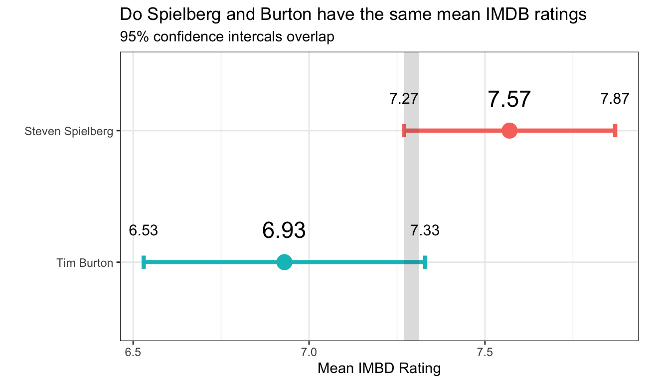
3. Hypothesis Testing using the t-test and “infer” package
Null hypotheses:the mean IMDB rating for Steven Spielberg and Tim Burton are the same .
Alternative hypotheses:the mean IMDB rating for Steven Spielberg and Tim Burton are not the same .
Using the t-test:
t.test(rating ~ director, data = movies)##
## Welch Two Sample t-test
##
## data: rating by director
## t = 3, df = 31, p-value = 0.01
## alternative hypothesis: true difference in means between group Steven Spielberg and group Tim Burton is not equal to 0
## 95 percent confidence interval:
## 0.16 1.13
## sample estimates:
## mean in group Steven Spielberg mean in group Tim Burton
## 7.57 6.93Using the infer package:
# Calculate diff in means

obs_diff <- movies %>%
  specify(rating ~ director) %>%
  calculate(stat = "diff in means", order = c("Steven Spielberg","Tim Burton"))


# Infer package

null_dist <- movies %>%
  # specify variables
  specify(rating ~ director) %>%

  # assume independence, i.e, there is no difference
  hypothesize(null = "independence") %>%

  # generate 1000 reps, of type "permute"
  generate(reps = 1000, type = "permute") %>%

  # calculate statistic of difference, namely "diff in means"
  calculate(stat = "diff in means", order = c("Steven Spielberg","Tim Burton"))

# Plot the relevant values

null_dist %>% visualize() +
  shade_p_value(obs_stat = obs_diff, direction = "two-sided")+
  theme_bw()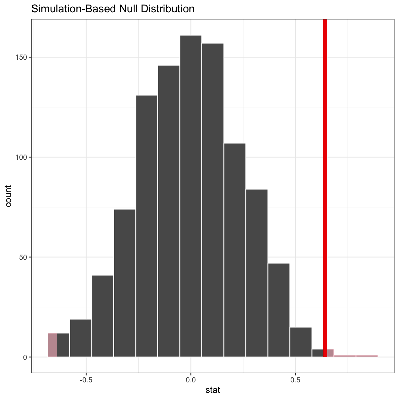
null_dist %>%
  get_p_value(obs_stat = obs_diff, direction = "two_sided")
## # A tibble: 1 × 1
## p_value
## <dbl>
## 1 0.008Answer:
Both the formula as well as the infer approach showed (p-value < 5% etc.) that we can reject the null hypothesis. At the end of the day we thus conclude that indeed the true difference in means between Steven Spielberg Movies and Tim Burton Movies is not equal to 0.